Part 2: Building an OEE Dashboard with FlowFuse

In Part 1, we explored the fundamentals of OEE, outlined a basic design of the dashboard, and identified the key elements to include in the OEE dashboard. In this Part 2, we will focus on building the OEE dashboard interface using FlowFuse Dashboard (Node-RED Dashboard 2.0) and FlowFuse, utilizing simulated production and downtime data.

# Getting Started

To simplify the development process, we will divide development into five key parts:

Collecting and configuring data
Preparing data for calculations
Calculating OEE and key metrics
Detailed breakdown of OEE data
Building the dashboard

Before we start, it is recommended to have a basic knowledge of Node-RED. For that, I recommend this free Node-RED Fundamental Course.

Additionally, ensure that you organize flows into well-structured groups. To match my group organization, I have provided images of the flow for each section. Also, if a Link In node is present at the start, create the group starting from the Link In node and ending at the Link Out node.

# Prerequisites

Before you begin building the OEE Dashboard with FlowFuse, make sure you have the following:

Running FlowFuse Instance: Make sure you have a FlowFuse instance set up and running. If you don't have an account, check out our free trial and learn how to create an instance in FlowFuse.
FlowFuse Dashboard: Ensure you have FlowFuse Dashboard (also known as Node-RED Dashboard 2.0 in the community) installed and properly configured on your instance.
SQLite Contrib Node: Ensure you have node-red-contrib-sqlite installed.

# Preparing Simulated Data

Before building the dashboard, we need a data source for production and downtime metrics. This data will serve as input for OEE calculations. We will focus on connecting a real source in the next part, but for now, let's generate simulated data.

Import the provided flow for data generation.
Click the Deploy button to activate the flow.
On deployment, it will create two SQLite tables: ProductionData and DowntimeData.
Find the Inject node labeled Click to generate and insert demo data.
Click the inject node to trigger data generation.

The flow will generate data with the following fields:

Demo Production and Downtime data object Demo Production and Downtime data object

# Collecting and Configuring Data

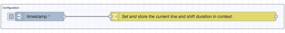
Once the simulated data is generated and stored in SQLite, the next step is to create a flow for configuration settings. These settings will be used across the entire flow, allowing the flow to be reused by simply modifying the settings. The configured data will then be collected for use in the OEE dashboard.

# Adding flow to configure settings:

Click on the "+" to create a new flow.
Name the newly created flow to OEE Dashboard for Line-1.
Drag a Change node onto the canvas, double-click it, and add the following elements:
- Set flow.line to "Line-1"
- Set flow.shift_duration to 12
- Set flow.shiftDuration24h to 24
Drag an Inject node, set it to trigger on deploy by enabling Inject once after X seconds (set delay to 0.1 seconds).
Click Deploy to apply changes.

In this flow, we are configuring the production line based on the demo data, specifically for Line-1, as we are building the OEE dashboard for this line. The settings define the shift duration for the last X hours used in OEE calculations and the total shift duration within a 24-hour period.

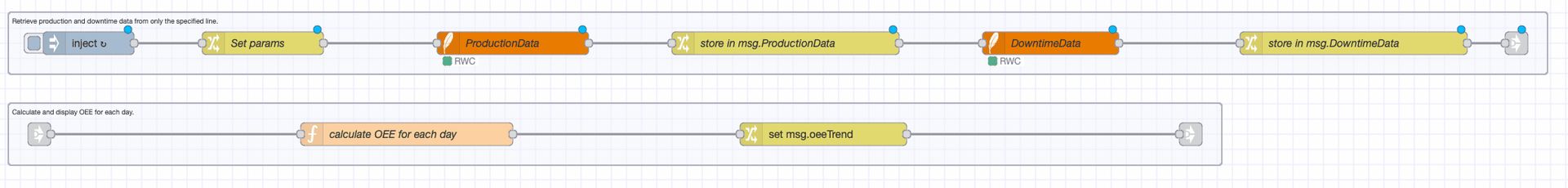
Flow to set basic configuration settings that will be used across the OEE dashboard flow for calculations. Flow to set basic configuration settings that will be used across the OEE dashboard flow for calculations.

# Retrieving Data from SQLite:

Drag an Inject node and configure it to trigger at regular intervals.
Drag a Change node and add following elements:
- Set msg.params to {}
- Set msg.params.$startTime to $moment($millis() - ($number($flowContext('shift_duration')) * 60 * 60 * 1000)).format('YYYY-MM-DD HH:mm:ss')
- Set msg.params.$endTime to $moment($millis()).format('YYYY-MM-DD HH:mm:ss')
- Set msg.params.$line to flow.line

Drag an SQLite node and insert the following query:

SELECT timestamp, machine_name, area, line, total_produced_units, good_units, defect_units, target_output
FROM ProductionData
WHERE timestamp BETWEEN $startTime AND $endTime AND line = $line;

Drag a Change node onto the canvas and set the following element to store the retrived production data result as new property:
- Set msg.payload to msg.productionData
Connect the Inject node’s output to the input of the Change node that sets parameters. Then, connect the Change node’s output to the input of the SQLite node that retrieves production data. Finally, connect the SQLite node’s output to the input of last change node we added.

Drag another SQLite node and insert the following query:

SELECT timestamp, machine_name, downtime_start, downtime_duration_minutes, downtime_reason
FROM DowntimeData
WHERE timestamp BETWEEN $startTime AND $endTime AND line = $line;

Drag a Change node onto the canvas and set the following element to store the retrived production data result as new property:
- Set msg.payload to msg.downtimeData
Connect the SQLite node’s output to the input of last change node we added.
Now, drag the Link Out node onto the canvas and connect it to the last Change node.

Flow that retrives the data from the sqlite table Flow that retrives the data from the sqlite table

# Preparing Data for OEE Calculations

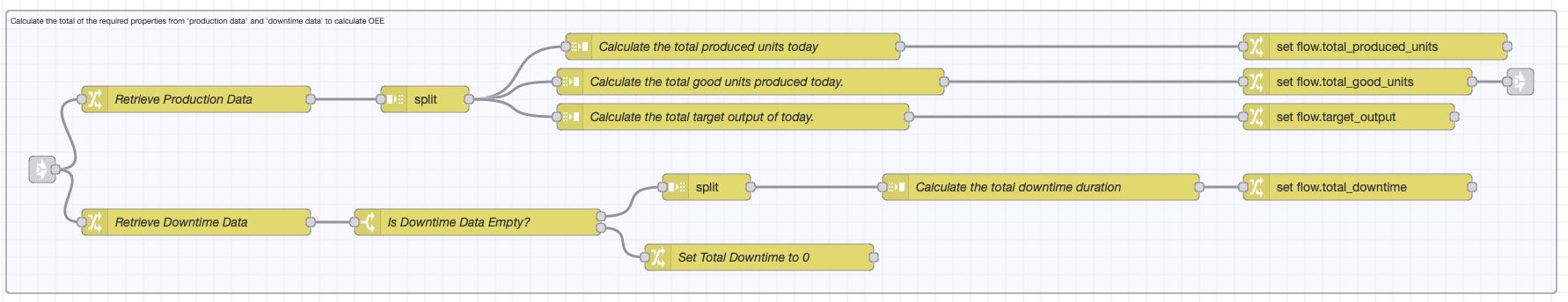
Now that we have a flow to retrieve production and downtime data, we can calculate key OEE metrics. The total number of good units, defective units, total produced units, target output, and downtime duration are summed across all production lines. Using these values, we can calculate availability, performance, and quality for the entire production system, which can then be used to calculate OEE.

Drag the link in node onto the canvas and connect it to the link out node.
Drag two Change nodes onto the canvas and connect them to the Link In node.
- In the first Change node, set msg.payload to production_data.
- In the second Change node, set msg.payload to downtime_data.
Drag a Split node onto the canvas and connect it to the first Change node, the one setting production_data. Configure the Split node so that msg.payload is assigned to production_data.
Drag three Join nodes onto the canvas and connect them to the Split node to sum individual data points. Configure each Join node with the following settings:
- Mode: Reduce Sequence
- Initial Value: 0
- Fix-up Expression: $A
Set the reduce expressions as follows:
- First Join Node: $A + msg.payload.total_produced_units
- Second Join Node: $A + msg.payload.good_units
- Third Join Node: $A + msg.payload.target_output
Drag three Change nodes onto the canvas and connect each to a Join node.
Configure these Change nodes to store the summed values using the following variables to flow context:
- total_produced_units
- total_good_units
- total_target_output
Drag a Switch node onto the canvas and connect it to the Change node that sets the retrieved downtime data to msg.payload, for switch node set the Property to msg.payload and add the following conditions:
- is not empty.
- Otherwise.
Drag a Split node onto the canvas and connect it to the first output of the Switch node.
Drag a Join node onto the canvas and connect it to the Split node.
Configure the Join node with the following settings:
- Mode: Reduce Sequence
- Initial Value: 0
- Fix-up Expression: $A
- Reduce Expression: $A + payload.downtime_duration_minutes
Drag a Change node onto the canvas and connect it to the Join node, Configure this Change node to store the total downtime duration in the flow context with following element:
- Set flow.total_downtime to msg.payload
Drag another Change node onto the canvas and connect it to the second output of the Switch node, Set this Change node to store 0 in the flow context for total_downtime with following element:

Set flow.total_downtime to 0

Drag a Link Out node onto the canvas and connect it to any of the Change nodes that store the summed metrics in the flow context.

Flow to prepare the data necessary to calculate OEE and all its three components. Flow to prepare the data necessary to calculate OEE and all its three components.

# Calculating OEE and Key Metrics

Now that we have all the necessary pieces, we can calculate the key metrics for OEE: Availability, Performance, and Quality and later OEE.

Drag a Link In node.
Drag a Change node and add element as following:
- Set msg.quality to ($flowContext('total_good_units') / $flowContext('total_produced_units')) * 100 as JSONata expression.
- Set msg.availability to (($flowContext('shift_duration') - $flowContext('total_downtime')) / $flowContext('shift_duration')) * 100 as JSONata expression.
- Set msg.performance to ($flowContext('total_produced_units') / $flowContext('target_output')) * 100 as JSONata expression.
- Set msg.oee to $round(((msg.availability / 100) * (msg.performance / 100) * (msg.quality / 100)) * 100, 2) as JSONata expression.
- Set msg.qualityto $round(msg.quality, 2)
- Set msg.availability to $round(msg.availability, 2)
- Set msg.performance to $round(msg.performance, 2)
- Set msg.productionData to JSONata expression:
```
[
{
    "reason": "Total Good Units Produced",
    "units": $flowContext("total_good_units")
  },
  {
    "series": "Total Defective Units Produced",
    "units": $number($flowContext("total_produced_units")) - $number($flowContext("total_good_units"))
  }
]
```
Drag a Link Out node and connect it to the Change node.
Drag a separate Link In node for visualization and keep it in a separate flow. This will be the Link In node where all the calculated final data for visualization will be stored.
Connect link out node to this link in node.

Flow that calculates availability, quality, performance, and OEE, and also prepares production data for visualization. Flow that calculates availability, quality, performance, and OEE, and also prepares production data for visualization.

# Detailed Breakdown of OEE Data

We have calculated the OEE and other key metrics. However, as discussed in the planning section of our previous article, we will also visualize recent downtime events, a downtime summary, the top underperforming machines (OEE-wise), and the OEE trend over the last 30 days on the dashboard.

Let’s do that.

Drag the link in node onto the canvas and connect it to the link out node that is part of the SQLite flow, which is also connected to the change node that sets the retrieved downtime result to msg.payload.
Drag a change node onto the canvas and set the following element: Set msg.downtime_data to msg.payload.

# Downtime Summary

Drag a function node onto the canvas and add the following JavaScript to calculate the downtime summary:

function calculateDowntimeByReason(downtimeData) {
   if (!Array.isArray(downtimeData) || downtimeData.length === 0) {
       return []; f
   }
   const summary = {};
   downtimeData.forEach(({ downtime_reason, downtime_duration_minutes }) => {
       summary[downtime_reason] = (summary[downtime_reason] || 0) + downtime_duration_minutes;
   });
   return Object.entries(summary).map(([reason, duration]) => ({
       downtime_reason: reason,
       downtime_duration_minutes: duration
   }));
}
msg.payload = calculateDowntimeByReason(msg.payload) || [];
return msg;

Drag a change node onto the canvas and set:
- Set msg.payload to msg.downtimeSummary.
Drag a link out node and connect it to the change node that sets msg.downtime_data to msg.payload.
Connect this link out node to the link in node that we added earlier to receive all the calculated metrics for visualization.

# Recent Downtime

Drag a Switch node onto the canvas and set the property to msg.payload. Add the following condition:
- is not empty
- otherwise
Drag a Split node onto the canvas and connect it to the first output of the Switch node.
Drag a Sort node onto the canvas and connect it to the Split node. Set the sort to "message sequence", key to msg.payload.downtime_start, and order to "descending." This will sort the downtime data from most recent to oldest based on its start time.
Drag a Join node onto the canvas and set the mode to automatic, then connect it to the Sort node.
Drag a Change node onto the canvas and set the following element:
- Set msg.recentDowntime to payload^(10) as a JSONata expression.
Connect the Change node to the Link Out node that was added before.

# Top Underperforming Machines

Drag a Function node onto the canvas and connect it to the Link In node that is receiving the SQLite result.
Add the following JavaScript code to the Function node:

const productionData = msg.production_data;
const downtimeEvents = msg.downtime_data;
const shiftDuration = (flow.get('shift_duration') || 1) * 60; // Convert hours to minutes

// Group production data by machine (including area)
let machineData = {};
productionData.forEach(data => {
    if (!machineData[data.machine_name]) {
        machineData[data.machine_name] = {
            total_produced_units: 0,
            good_units: 0,
            target_output: 0,
            count: 0,
            area: data.area // Store area
        };
    }
    machineData[data.machine_name].total_produced_units += data.total_produced_units;
    machineData[data.machine_name].good_units += data.good_units;
    machineData[data.machine_name].target_output += data.target_output;
    machineData[data.machine_name].count += 1;
});

let oeeResults = Object.keys(machineData).map(machineName => {
    let data = machineData[machineName];

    let machineDowntime = downtimeEvents.filter(event => event.machine_name === machineName);

    function calculateOEE(data, downtime) {
        if (data.target_output === 0) {
            return { availability: 0, performance: 0, quality: 0, oee: 0 };
        }

        let totalDowntime = downtime.reduce((acc, event) =>
            typeof event.downtime_duration_minutes === 'number' ? acc + event.downtime_duration_minutes : acc
            , 0);

        let availability = (shiftDuration - totalDowntime) / shiftDuration;
        availability = Math.max(0, Math.min(1, availability));

        let performance = data.target_output > 0 ? data.total_produced_units / data.target_output : 0;
        let quality = data.total_produced_units > 0 ? data.good_units / data.total_produced_units : 0;

        let oee = availability * performance * quality;

        return {
            availability: parseFloat((availability * 100).toFixed(2)),
            performance: parseFloat((performance * 100).toFixed(2)),
            quality: parseFloat((quality * 100).toFixed(2)),
            oee: parseFloat((oee * 100).toFixed(2))
        };
    }

    let metrics = calculateOEE(data, machineDowntime);

    return {
        machine_name: machineName,
        area: data.area,
        oee: metrics.oee
    };
});

// Filter only machines with OEE < 85
msg.payload = oeeResults.filter(machine => machine.oee < 85);

return msg;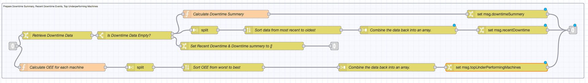

Flow that prepares the Recent Downtime, Downtime Summary, and Top Underperforming Machines (OEE-wise) Flow that prepares the Recent Downtime, Downtime Summary, and Top Underperforming Machines (OEE-wise)

# OEE Trend for the Last 30 Days

Now, to calculate the OEE for the last 30 days, we need the complete production and downtime data for that period. However, the current SQLite flow retrieves only the last 12 hours. Therefore, we need another SQLite flow to retrieve data from the last 30 days.

# Retrieving Production and Downtime Data for the Last 30 Days

Copy the existing SQLite flow from the Inject node to the Change node that sets the retrieved downtime result to msg.payload.
Click on the Change node that sets the parameters for the SQL query, keep only the element setting the line parameter, and remove the rest.
Modify the first SQLite node's SQL query to the following:

SELECT
    timestamp AS timestamp,
    machine_name AS machine_name,
    area AS area,
    line AS line,
    total_produced_units AS total_produced_units,
    good_units AS good_units,
    defect_units AS defect_units,
    target_output AS target_output
FROM ProductionData
WHERE line = $line
  AND timestamp >= datetime('now', '-30 days');

Modify the second SQLite node's SQL query to the following:

SELECT
    timestamp AS timestamp,
    machine_name AS machine_name,
    downtime_start AS downtime_start,
    downtime_duration_minutes AS downtime_duration_minutes,
    downtime_reason AS downtime_reason
FROM DowntimeData
WHERE
    timestamp BETWEEN $startTime AND $endTime
    AND line = $line;

# Calculating last 30d days OEE

Drag the Link Out node onto the canvas and connect it to the last Change node of the SQLite flow.
Drag the Link In node onto the canvas and connect it to the last Link Out node.
Drag the Function node onto the canvas, add the following JavaScript, and connect the Function node to the Link In node:

let productionData = msg.production_data;
let downtimeData = msg.downtime_data;
let line = flow.get('line');
let shiftDuration = flow.get('shiftDuration24h') * 3600;

let groupedData = {};

productionData.forEach(entry => {
    if (entry.line === line) {
        let date = entry.timestamp.split(" ")[0];

        if (!groupedData[date]) {
            groupedData[date] = {
                totalShiftDuration: shiftDuration,
                totalGoodUnits: 0,
                totalProducedUnits: 0,
                totalDowntimeSeconds: 0,
                totalCycleTime: 0,
                cycleCount: 0,
                totalTargetOutput: 0,
                timestamp: entry.timestamp
            };
        }

        groupedData[date].totalGoodUnits += entry.good_units;
        groupedData[date].totalProducedUnits += entry.total_produced_units;
        groupedData[date].totalCycleTime += entry.cycle_time;
        groupedData[date].cycleCount++;
        groupedData[date].totalTargetOutput += entry.target_output;
    }
});

downtimeData.forEach(downtime => {
    if (downtime.line === line) {
        let date = downtime.timestamp.split(" ")[0];
        if (groupedData[date]) {
            groupedData[date].totalDowntimeSeconds += downtime.downtime_duration_minutes * 60;
        }
    }
});

let oeeResults = Object.entries(groupedData).map(([date, data]) => {
    let avgCycleTime = data.cycleCount > 0 ? data.totalCycleTime / data.cycleCount : 0;
    let availableTime = data.totalShiftDuration - data.totalDowntimeSeconds;
    let availability = availableTime / data.totalShiftDuration;
    let performance = data.totalTargetOutput > 0 ? data.totalProducedUnits / data.totalTargetOutput : 0;
    let quality = data.totalProducedUnits > 0 ? data.totalGoodUnits / data.totalProducedUnits : 0;
    let oee = (availability * performance * quality * 100).toFixed(2);

    return { date, availability, performance, quality, oee, timestamp: data.timestamp };
});

// Sort data by timestamp (oldest to most recent)
oeeResults.sort((a, b) => new Date(a.timestamp).valueOf() - new Date(b.timestamp).valueOf());
msg.payload = oeeResults;
return msg;

Drag the Change node onto the canvas and set msg.payload to msg.oeeTrend.
Drag the Link Out node onto the canvas and connect it to the Change node.
Connect this Link Out node to the Link In node that was added earlier to receive all the calculated metrics for visualization.

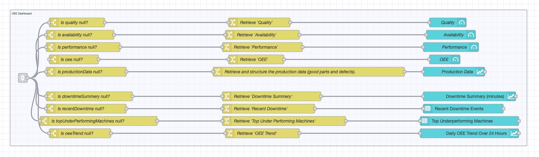
Flows that calculate the OEE for each day over the last 30 days Flows that calculate the OEE for each day over the last 30 days.

# Building the OEE Dashboard

Now that the key OEE metrics have been calculated and detailed insights into production performance have been gathered, it is time to bring everything together in a visually intuitive and interactive dashboard. The OEE dashboard will provide real-time visibility into availability, performance, and quality while also displaying recent downtime events, downtime summaries, underperforming machines, and historical OEE trends.

Using FlowFuse Dashboard (Node-RED Dashboard 2.0), a clean and efficient interface will be designed, allowing operators and decision-makers to monitor production efficiency at a glance.

Drag a Switch node onto the canvas, set the property to msg.oee, and add the condition:
- "Is not null".
Connect it to the Link-In node that receives calculated metrics.
Drag a Change node, set msg.oee to msg.payload, and connect it to a Gauge widget.
- Create a new Group on a new page named Line-1.
- Set the page layout to Grid, adjust the range from 0 to 100, and label the gauge OEE.
- Choose Half Gauge as the type, set the style to Rounded, and adjust the width and height to 6 and 3 for both the group and the widget.
Repeat these steps for msg.quality, msg.availability, and msg.performance, ensuring each has a separate Group with the correct label.
Drag a Switch node for msg.productionData and connect it to a Change node setting msg.productionData to msg.payload:
- "Is not null".
Repeat this step for msg.downtimeSummary, msg.recentDowntime, msg.topUnderPerformingMachines, and msg.oeeTrend, ensuring each has a separate Switch node and Change node.
Drag a Bar Chart widget, create a new Group, set the width to 6 and height to 8 for both the group and widget, label it Production Data, group data by Stacks, and map X to series and Y to units. Connect it to the node setting msg.productionData.
Duplicate the chart for Downtime Summary, mapping X to downtime_reason and Y to downtime_duration_minutes, and connect it to the node setting msg.downtimeSummary to msg.payload.
Drag a Table widget, create a new Group, set width 6 and height 2 for both the group and widget, label it Recent Downtime Events, set max rows to 5, and add columns with keys:
- machine_name
- downtime_start
- downtime_duration_minutes
- downtime_reason
Connect it to the node setting msg.recent_downtime to msg.payload.
Duplicate the table for Top Underperforming Machines, adding columns with keys:
- machine_name
- area
- oee
Connect it to msg.topUnderPerformingMachines.
Drag a Line Chart widget, create a new Group, set width 12 and height 5 for both the group and widget, label it Daily OEE Trend Over 24 Hours, set X-axis to Timescale, format Y-l-d, and map X to date and Y to oee. Connect it to the Change node setting msg.oeeTrend to msg.payload.
Click Deploy.
Open the dashboard by clicking the Dashboard 2.0 button located at the top-right corner of the Dashboard 2.0 sidebar.

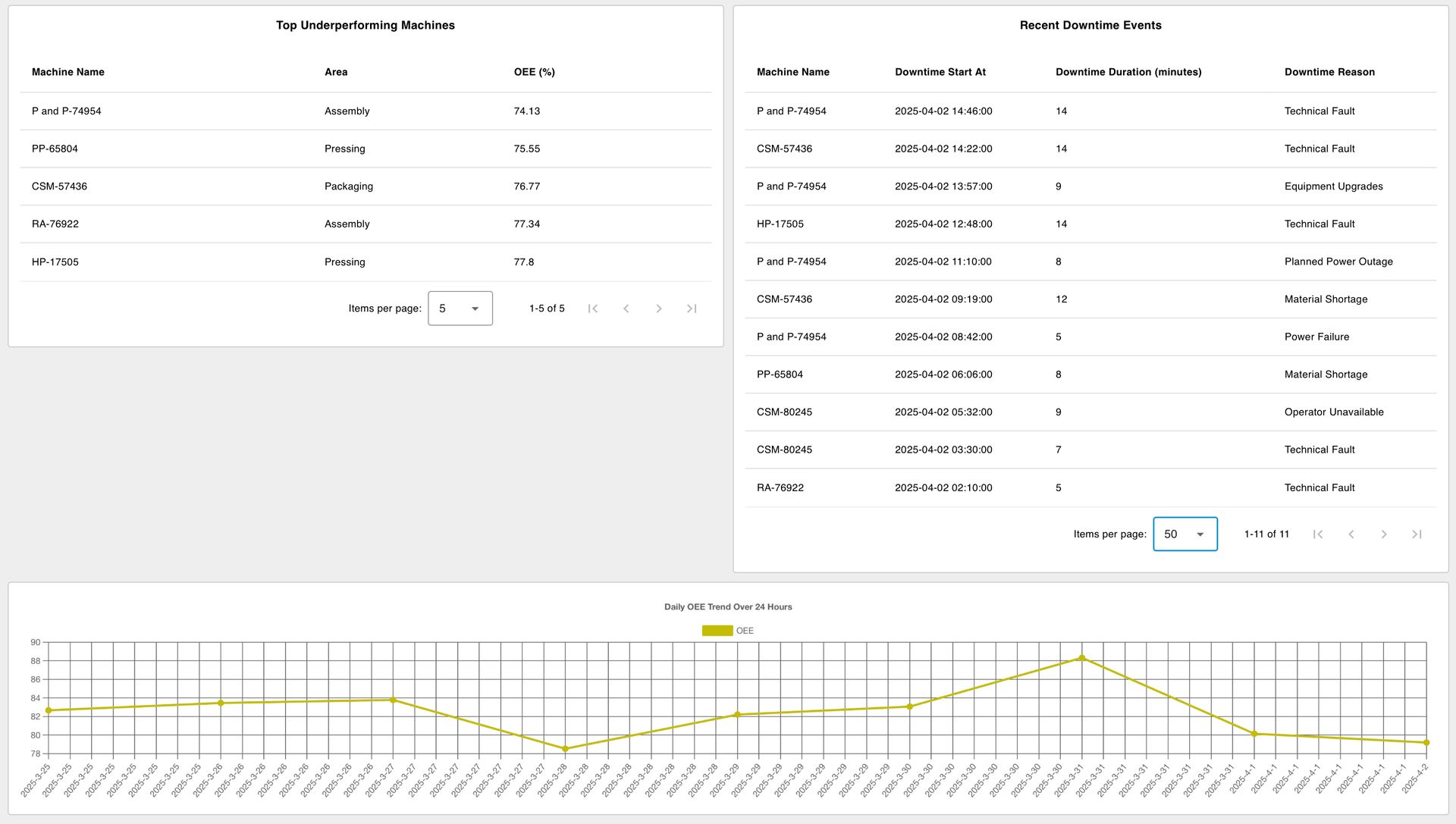
OEE Dashboard UI flow OEE Dashboard UI flow

Your OEE dashboard is now set up and ready to use. It will visualize key metrics, including OEE, quality, availability, performance, production data, downtime events, and machine performance trends.

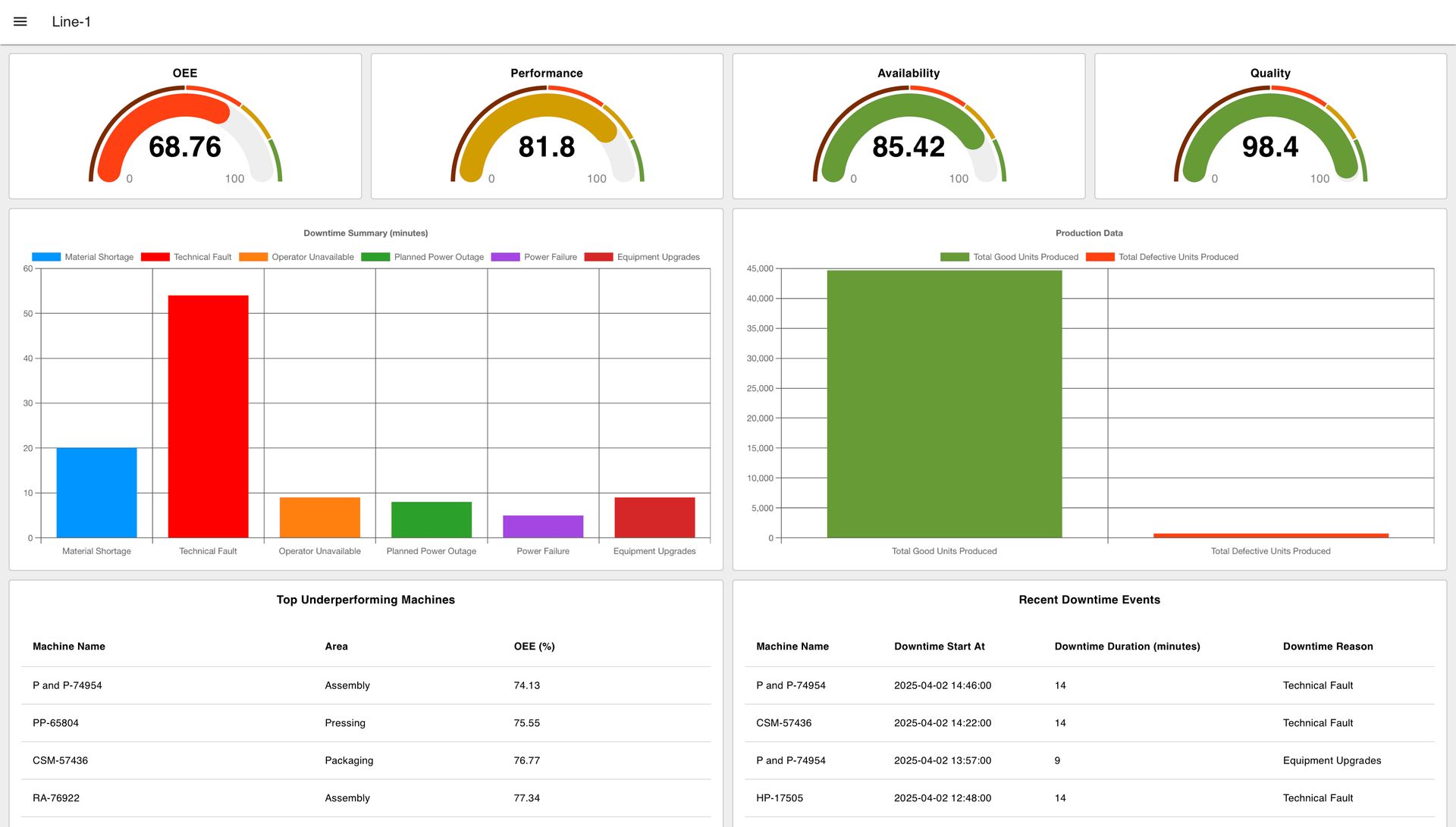
OEE Dashboard results without proper theming and styling OEE Dashboard results without proper theming and styling.

OEE Dashboard results without proper theming and styling OEE Dashboard results without proper theming and styling

However, the dashboard may not yet look exactly as it did in the previous design or intended layout. Some components may not align correctly with adjacent components in terms of width and height. Additionally, on different screens, you may notice layout inconsistencies, and the top header elements, such as the OEE Dashboard title and logo is missing.

Do not worry—in the next part of this series, we will style the dashboard to match the original design. Later, we will demonstrate how to connect it to a real data source, scale it across your production lines, and explain how you can use this dashboard to improve production efficiency.

# What Next?

Part 3 of this series will follow soon. In the meantime, if you’re excited to quickly launch your OEE dashboard in your factory environment, don’t delay! Register for a FlowFuse account now and initiate your journey with our new effective, ready-made OEE Dashboard Blueprint.

Step-by-step guide to building your own OEE Dashboard.