Building Historical Data Dashboard with FlowFuse Tables
Collect, transform, store and visualize IIoT data using FlowFuse Tables
In Industrial IoT, tracking data over time is crucial. Whether you’re monitoring temperature changes throughout the day, spotting machine downtime, or analyzing production trends across shifts, a historical data dashboard helps you see important patterns clearly.
This tutorial guides you through building such a dashboard using FlowFuse Tables. FlowFuse Tables currently provides a managed PostgreSQL database—a reliable and widely used system—which we will use throughout this tutorial to store time-series data.
Why PostgreSQL for Time-Series Data?
You might wonder if PostgreSQL can efficiently handle large volumes of time-series data. The answer is yes—when configured properly. Without optimization, query performance can slow as data grows. However, by using techniques like batch inserts and smart indexing, PostgreSQL delivers fast and reliable access even at an industrial scale.
PostgreSQL is selected as the first database offering in FlowFuse Tables because it is flexible, reliable, and open source. It serves as a solid foundation for FlowFuse Tables. Whether your data comes from IIoT sensors or other sources, PostgreSQL is well equipped to handle it.
Prerequisites
Before we begin, please ensure you have the following set up:
- A FlowFuse Enterprise account, as FlowFuse Tables is an exclusive Enterprise feature.
- The
@flowfuse/node-red-dashboardpackage installed in your FlowFuse instance to create the user interface. - The
node-red-contrib-momentnode installed for handling date and time operations within your flows. - FlowFuse Tables configured for your FlowFuse Team with a managed PostgreSQL database.
If you are new to FlowFuse Tables, we highly recommend reading our getting started guide to familiarize yourself with the basics.
Creating an Optimized Database Schema
Our first step is to design a database table structured for both high-speed writes and efficient queries.
Step 1: Design and Create the Table
We will create a single table to hold all our sensor data. The key is to use appropriate data types and indexes to ensure performance.
-
In your FlowFuse Node-RED instance, drag a Query node onto the canvas.
-
Configure the node with the following SQL statement to create the table and its indexes:
CREATE TABLE "sensor_readings" (
    "id" SERIAL PRIMARY KEY,
    "timestamp" TIMESTAMPTZ NOT NULL DEFAULT NOW(),
    "sensor_id" VARCHAR(50) NOT NULL,
    "location" VARCHAR(100),
    "temperature" DECIMAL(5,2)
);

CREATE INDEX "idx_sensor_timestamp" ON "sensor_readings"("sensor_id", "timestamp" DESC);
Schema Breakdown:
TIMESTAMPTZ: We use this data type to store timestamps with timezone information. This is critical for applications with sensors spread across different geographical locations, ensuring data is always consistent.- Index: The composite index on
sensor_idandtimestamp(in descending order) is vital for query speed. It allows PostgreSQL to quickly locate and return results for a specific sensor while already ordering them from newest to oldest. This avoids expensive sorting when fetching the most recent readings for a given sensor.
Important: The
DESCin the composite index provides a significant performance boost for queries like:SELECT *
FROM sensor_readings
WHERE sensor_id = 'sensor_01'
ORDER BY timestamp DESC
LIMIT 10;If you instead need results in chronological order, you could create an ascending index or let PostgreSQL reverse the order at query time.
- To execute this one-time setup, connect an Inject node to the input of the Query node and a Debug node to its output.
- Click Deploy, then click the button on the Inject node to create your table.
Step 2: Storing Sensor Data Efficiently with Batch Inserts
Writing every single sensor reading to the database individually can create significant overhead and slow down performance. A much more efficient method is to "batch" readings together and write them in a single transaction.
Let's build a flow to simulate sensor data and batch-insert it.
-
Add an Inject node configured to repeat every 1 second to simulate a continuous stream of data.
-
Connect it to a Change node that generates a simulated sensor reading. Configure it to set
msg.payloadusing the following JSONata expression:
    {
        "sensor_id": "sensor_01",
        "location": "Production Line A",
        "temperature": 20 + $random() * 5
}-
Add another Change node to add a precise timestamp to each reading.
- Set
msg.payload.timestamp - To the value type timestamp.
- Set
-
Add a Function node and name it "Batch Accumulator". Paste the following JavaScript code into the node — it already includes inline comments explaining each step. This function will accumulate incoming readings in batches until the specified batch size is reached, and then creates the SQL query to perform batch inserts into the database.
// Set the number of records to collect before triggering a batch insert
const batchSize = 100;

// Retrieve previously stored readings from context (or start with an empty array)
const readings = context.get('readings') || [];

// Add the new reading (from msg.payload) to the readings array
readings.push(msg.payload);

// Check if we have enough readings to perform a batch insert
if (readings.length >= batchSize) {

    // Generate parameter placeholders for each reading (4 fields per record)
    // Example: ($1, $2, $3, $4), ($5, $6, $7, $8), ...
    const values = readings.map((_, i) =>
        `($${i * 4 + 1}, $${i * 4 + 2}, $${i * 4 + 3}, $${i * 4 + 4})`
    ).join(',');

    // Build the SQL insert query with placeholders
    msg.query = `
        INSERT INTO sensor_readings
        (timestamp, sensor_id, location, temperature)
        VALUES ${values};
    `;

    // Flatten the readings into a single array of values matching the placeholders
    // For each reading, we pass: current timestamp, sensor_id, location, temperature
    msg.params = readings.flatMap(r => [
        new Date(),          // Or use r.timestamp if actual reading time is available
        r.sensor_id,
        r.location,
        r.temperature
    ]);

    // Clear stored readings in context now that they are being inserted
    context.set('readings', []);

    // Return the msg with the SQL query and parameters for execution
    return msg;
}

// If not enough readings collected yet, store them back into context
context.set('readings', readings);

// Do not send anything forward yet
return null;-
Connect the output of the "Batch Accumulator" to a Query node. This node will receive the fully formed
msg.queryand execute the batch insert. -
Deploy the flow. It will now collect 100 readings (over 100 seconds) and perform a single, highly efficient database write instead of 100 separate ones.
Building the Interactive Dashboard
With data flowing into our database, let's create a user interface to query and visualize it.
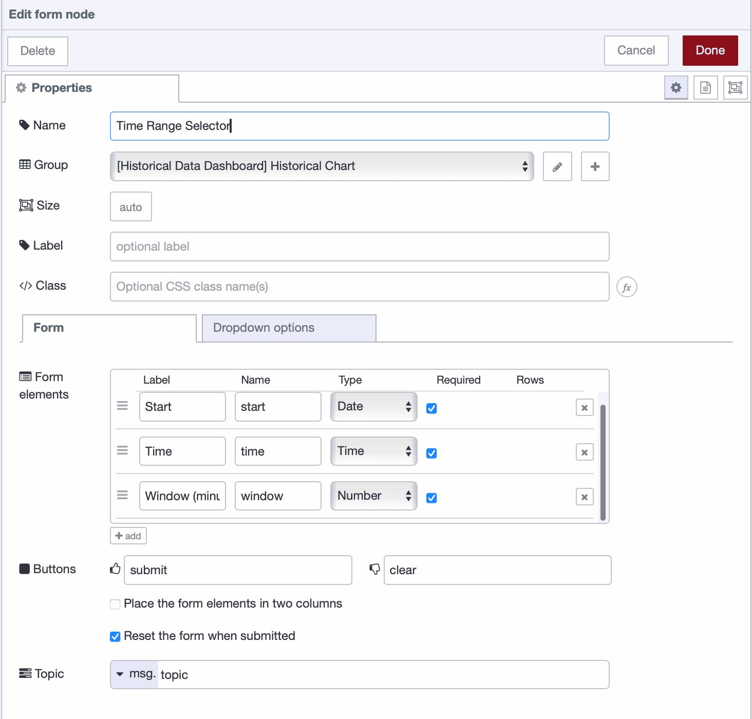
Step 3: Create an Interactive Time Range Selector
We'll start with a form that allows users to select a date, time, and duration to view.
-
Drag a ui_form node onto the canvas. Create a new dashboard group for it and add the following form elements:
-
Connect the output of the form to a Change node to format the input. Add the following rules in the Change node:
-
Set
msg.startDateTimeto the JSONata expression:payload.start & "T" & payload.time & ":00" -
Set
msg.windowMinutesto the expression:payload.window
-
-
Add a Date/Time Formatter node. This is crucial for handling timezones correctly. Configure it as follows:
- Input property:
msg.startDateTime - Input timezone: your local timezone, for example,
Asia/Kolkata - Output timezone:
Etc/UTC(to match the databaseTIMESTAMPTZstandard) - Output property:
msg.startDateTime
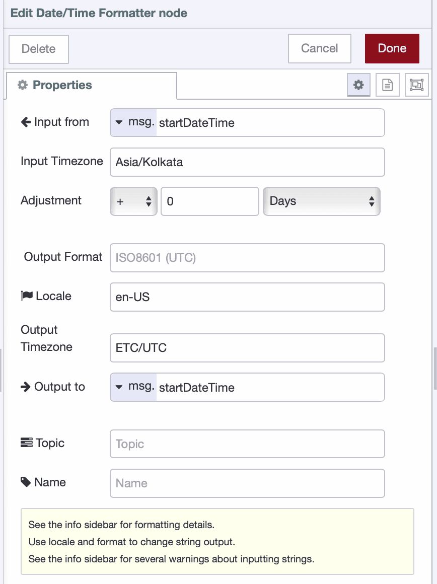
- Input property:
-
Add another Change node to set the query parameters for the SQL query. Set
msg.paramsto the following JSONata expression:[ msg.startDateTime, msg.windowMinutes & " minutes" ] -
Connect this to a Query node with the following parameterized SQL, which fetches data for the selected time window:
SELECT
    "timestamp",
    "temperature"
FROM "sensor_readings"
WHERE "sensor_id" = 'sensor_01'
  AND "timestamp" >= $1::timestamptz
AND "timestamp" < ($1::timestamptz + $2::interval) ORDER BY "timestamp" DESC; -
Connect a Debug node after the Query node to test the flow.
-
Drag a Switch node onto the canvas and add a condition to check whether
msg.payloadis empty. Connect the output of the Query node to the Switch node. -
Connect the output for the "empty" condition from the Switch node to a Change node that sets
msg.payloadto:No data found for the selected time range. -
Drag a ui_notification node, select the appropriate UI group, and connect it to the output of the Change node.
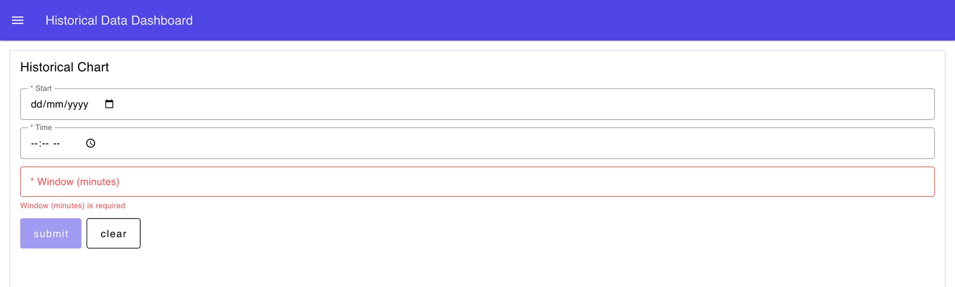
-
Deploy the flow. On the dashboard, select a date, time, and window using the form. Verify in the debug panel that the correct data is returned, or that a notification appears if no data is found.
Step 4: Display the Data in a Chart
The final step is to visualize the query result.
-
Connect the output of the final Query node to a ui_chart widget.
-
Configure the chart node:
- Group: Create new group for chart.
- Type: Line
- X: Set to
timestampas a key. - Y: Set to
temperatureas a key. - Series: Set to "Temperature" as string.
-
Deploy the flow. Your complete historical data dashboard is now live — you can explore it and experiment with different time ranges to see the results.

Below is the complete flow we built in this tutorial.
Conclusion
You have successfully built a historical data dashboard using FlowFuse Tables and Node-RED. By implementing efficient batch inserts and optimized query patterns, you have created a solution that is both powerful and scalable for demanding Industrial IoT environments.
With FlowFuse Tables now part of the platform, you can build complete industrial applications without juggling external databases or leaving the FlowFuse environment. FlowFuse is now a comprehensive data platform with the ability to collect, connect, transform, store, and visualize data. Combined with FlowFuse's enterprise features—team collaboration, version control, device management, and secure deployments—you have everything needed to take your IIoT projects from prototype to production within one integrated platform.
This means less complexity and faster time to value for your industrial data initiatives. Your historical dashboards, real-time monitoring, and OEE dashboards can all live in the same ecosystem, managed by the same team, with consistent security and governance controls.
Ready to build your own time-series dashboard? Get started with FlowFuse Tables or explore our industrial blueprints
Discuss your use case with our team
See how FlowFuse can support your architecture, integrations, and deployment needs.
About the Author
Sumit Shinde
Technical Writer
Sumit is a Technical Writer at FlowFuse who helps engineers adopt Node-RED for industrial automation projects. He has authored over 100 articles covering industrial protocols (OPC UA, MQTT, Modbus), Unified Namespace architectures, and practical manufacturing solutions. Through his writing, he makes complex industrial concepts accessible, helping teams connect legacy equipment, build real-time dashboards, and implement Industry 4.0 strategies.